Wednesday, September 26, 2007

Meeting update Wednesday September 26

I held a meeting today with Dr.Poon to discuss my progress to date. The majority of the meeting was centered around how we were going to obtain the p-values for the implied values in the aggregation tests that I mentioned in my earlier post. Dr. Poon informed me that Shazam (another statistical package) has the ability to calculate the p-values for the implied delta and gamma values obtained. We have decided to use the Shazam software for the portion of this thesis. I have been provided with a copy of Shazam and have already installed the software, written the the code to perform the tests and obtained the results.

The code that I wrote to perform the aggregation tests is quite simple and is provided below.

*Read in the Data
SAMPLE 1 216
READ(AggregationData89_06.txt) Sector KH KS K1 K KSITP KSP KHP K0 L VA / SKIPLINES=1

*Transform Variables
GENR KSP = LOG(KSP)
GENR KHP = LOG(KHP)
GENR KSITP = LOG(KSITP)

GENR VA=LOG(VA)
GENR L=LOG(L)
GENR K=LOG(K)
GENR K1=LOG(K1)
GENR K0=LOG(K0)
GENR KS=LOG(KS)
GENR KH=LOG(KH)

*Create time effect dummies
MATRIX TDUM=SEAS(216,18)
DO #=1,18
GENR C#=TDUM:#
ENDO

* Run OLS for first aggregation test
OLS VA L K KSP KHP Sector C2-C18

*Perform the t-tests for the implied values
TEST
TEST K/KSP
END

TEST
TEST K/KHP
END

* Run OLS for the second aggregation test
OLS VA L K0 KSITP K1 Sector C2-C18

*Perform t-test for the implied value
TEST
TEST K1/KSITP
END

STOP

As is evident in the code above I had run the OLS by also using the natural log of the mix functions KSP (KS/K), KHP (KH/K) and KSITP (KS/K1). However, this provided an unexpected result in the first aggregation test with the p-value of the mix function KSP to be around 0.70 which means that since we cannot reject the null hypothesis from KSP being statistically different from zero this implies that KS (Software capital) can be aggregated into ordinary capital. I have passed on these results to Dr. Poon who has asked me to re-run the tests without taking the natural logs of these mix functions. The results now show that Software Capital (KS) and Hardware Capital (KH) cannot be aggregated with non-IT capital since the p-values of the mix functions KSP, KHP are less than 0.05. Likewise the second aggregation test results show that KS and KH cannot be aggregated into a single IT capital measure (K1) since the mix function KSITP has a p-value less than 0.01. The full results are posted below.

Test for aggregation of KS into K

TEST VALUE = 0.25394E-01 STD. ERROR OF TEST VALUE 0.12112E-01

T STATISTIC = 2.0966614 WITH 193 D.F. P-VALUE= 0.03733

F STATISTIC = 4.3959891 WITH 1 AND 193 D.F. P-VALUE= 0.03733

WALD CHI-SQUARE STATISTIC = 4.3959891 WITH 1 D.F. P-VALUE= 0.03602

Test for aggregation of KH into K

TEST VALUE = 0.78809E-02 STD. ERROR OF TEST VALUE 0.33973E-02

T STATISTIC = 2.3197322 WITH 193 D.F. P-VALUE= 0.02140

F STATISTIC = 5.3811575 WITH 1 AND 193 D.F. P-VALUE= 0.02140

WALD CHI-SQUARE STATISTIC = 5.3811575 WITH 1 D.F. P-VALUE= 0.02036


Test for aggregation of KS into K1

TEST VALUE = -0.18831 STD. ERROR OF TEST VALUE 0.23904E-01

T STATISTIC = -7.8779472 WITH 193 D.F. P-VALUE= 0.00000

F STATISTIC = 62.062051 WITH 1 AND 193 D.F. P-VALUE= 0.00000

WALD CHI-SQUARE STATISTIC = 62.062051 WITH 1 D.F. P-VALUE= 0.00000


I have passed on these results to Dr.Poon and am awaiting confirmation that I can report these results in my final report.


Tuesday, September 25, 2007

Aggregation Test Procedure

In my last post I mentioned that I was undertaking an aggregation test on the production inputs of software capital, hardware capital and non-IT capital to see if they can be combined into a single measure. I had performed this test but Dr. Poon had asked me to slightly adjust the model which I was using in the test which is based on Stiroh and McGukin (2002) aggregation paper. I am testing for two effects which are:

  1. If software and hardware capital can be aggregated into a single measure called IT capital
  2. If software, hardware and non-IT capital can be aggregated into a single capital measure


In either situation these separate capital items can be aggregated if they are perfect substitutes for each other and i.e. implies that the composition of these different capital measures are not important as the different components can be perfectly replaced by another component. E.g. if software capital and hardware capital can be aggregated into IT capital, IT capital would give the same result if it was 100% software capital, 50% hardware capital and 50% software capital etc. The first aggregation test, tests to see if the concepts of hardware and software capital are different. The second aggregation test tests to see if the concept of IT capital is different from the standard definition of ordinary capital.

The models to estimate are as follows:


Where:

KS is software capital

KH is hardware capital

L is labour

K1 is KS+KH, i.e. IT capital

K0 is non-IT capital

K is K0+KS+KH, aggregate capital

T, I control for time and sector effects

Initially I had used a restricted F-test on both models in accordance with Aizcorbe (1990) who proposed the aggregation test to see if these variables can be aggregate. A rejection of the null hypothesis of the restricted f-test means they are not aggregates and I rejected the null in both cases. However, Dr. Poon has asked me to calculate the implied gamma and delta values in addition to each variables p-value. Whilst it is simple to calculate the implied values by dividing b2 or b3 by b0 the p-value is more difficult since we don’t know the standard error of the implied value obtained by division. Dr. Poon said that we will work on this tomorrow in our meeting using some of the inbuilt functions in shazam as I have not found a function in R that will assist in calculating the p-value.

However, I might be able to determine the p-value of the implied coefficient via the following procedure. First I will run a regression of the proportional variable on the dependent variable:


Second, I will then use the fitted value obtained as a replacement for the regressor of the original model and re-run the regression.


Now not only will I have and estimate of the delta value as well as its standard error and will now be able to calculate the p-vale. However, I am not too sure if this will be valid as the implied value of delta should be obtained by the procedure I mentioned earlier. Nevertheless I will ask Dr.Poon if this procedure can be used in tomorrows meeting. After my meeting I will post up the details of which procedure was used to obtain the p-values of the implied delta and gamma values.

Monday, September 17, 2007

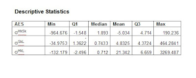
AES Descriptive Statistics

The previous post had some of the results descriptive statistics for each AES calculated, that is:

  • Software Capital and Hardware Capital
  • Software Capital and Labour
  • Hardware Capital and Labour

cut off. I have included it again in its entirety in this post.

On the Home Stretch

My meeting last week with Dr.Poon provided further clarity for the way going forward as to which data set is going to be used for the final AES results calculation and interpretation. In my last post I mentioned that data could be possibly modified by omitting an industry or removing outliers from the sample via an examination of the regression residuals. However Dr. Poon and I decided against either method owing to the fact the data has been obtained from the ABS. Thus, we do not expect there to be any observations that would adversely influence our results which could be expected in a case where we would have collected the data ourselves via surveys and other sources. Dr.Poon has also provided a data set for years form 2002-2006. Therefore the AES calculations and analysis is going to be conducted on the data from 1989-2006 across 12 industries.


I have included the results obtained for the regression, AES calculation for Software Capital and Hardware Capital (SKHK), Software Capital and Labout (SKL) and Hardware Capital and Labour (HKL) and the descriptive statistics of the AES calculated below.


REGRESSION RESULTS 1989-2002

Call:

lm(formula = data$lnVA ~ data$lnKS + data$lnKH + data$lnK0 +

data$lnL + KSKH + KSK0 + KSL + KHK0 + KHL + K0L + KS2 + KH2 +

K02 + L2 + factor(data$Time) + factor(data$Sector))

Residuals:

Min 1Q Median 3Q Max

-0.423377 -0.053865 0.007137 0.064163 0.236467

Coefficients:

Estimate Std. Error t value Pr(>|t|)

(Intercept) -2.76934 3.49685 -0.792 0.429738

data$lnKS -4.91899 0.73396 -6.702 4.73e-10 ***

data$lnKH 3.28292 0.43660 7.519 6.17e-12 ***

data$lnK0 -3.70208 0.62895 -5.886 2.82e-08 ***

data$lnL 6.46639 0.80948 7.988 4.68e-13 ***

KSKH 0.25449 0.07029 3.621 0.000411 ***

KSK0 0.31770 0.06177 5.143 9.01e-07 ***

KSL 0.29704 0.04364 6.807 2.74e-10 ***

KHK0 -0.22608 0.03697 -6.115 9.20e-09 ***

KHL -0.16539 0.02900 -5.702 6.82e-08 ***

K0L -0.37694 0.04122 -9.145 6.61e-16 ***

KS2 -0.21684 0.04987 -4.348 2.64e-05 ***

KH2 -0.05881 0.02768 -2.124 0.035406 *

K02 0.33207 0.04276 7.766 1.60e-12 ***

L2 -0.13565 0.02377 -5.708 6.65e-08 ***

factor(data$Time)2 -0.13121 0.04744 -2.766 0.006446 **

factor(data$Time)3 -0.24256 0.04959 -4.891 2.74e-06 ***

factor(data$Time)4 -0.32922 0.05204 -6.327 3.21e-09 ***

factor(data$Time)5 -0.36548 0.05353 -6.828 2.46e-10 ***

factor(data$Time)6 -0.38471 0.05436 -7.078 6.62e-11 ***

factor(data$Time)7 -0.39591 0.05481 -7.223 3.05e-11 ***

factor(data$Time)8 -0.37964 0.05574 -6.811 2.68e-10 ***

factor(data$Time)9 -0.37973 0.05732 -6.625 7.03e-10 ***

factor(data$Time)10 -0.36279 0.06060 -5.987 1.73e-08 ***

factor(data$Time)11 -0.39968 0.06408 -6.237 5.02e-09 ***

factor(data$Time)12 -0.46585 0.07016 -6.640 6.53e-10 ***

factor(data$Time)13 -0.57207 0.07291 -7.846 1.03e-12 ***

factor(data$Time)14 -0.61339 0.07620 -8.050 3.33e-13 ***

factor(data$Sector)1 0.50895 0.03061 16.628 <>

---

Signif. codes: 0 '***' 0.001 '**' 0.01 '*' 0.05 '.' 0.1 ' ' 1

Residual standard error: 0.1126 on 139 degrees of freedom

Multiple R-Squared: 0.9663, Adjusted R-squared: 0.9595

F-statistic: 142.4 on 28 and 139 DF, p-value: <>


AES RESULTS 1989-2002

σKSKH -5.033649

t = -0.8299, df = 167, p-value = 0.2039

alternative hypothesis: true mean is less than 0

95 percent confidence interval:

-Inf 4.998998

sample estimates:

mean of x

-5.033649

σKHL 21.34182

t = 1.0949, df = 167, p-value = 0.1376

alternative hypothesis: true mean is greater than 0

95 percent confidence interval:

-10.89738 Inf

sample estimates:

mean of x

21.34182

σKSL 4.832529

t = 1.7212, df = 167, p-value = 0.04353

alternative hypothesis: true mean is greater than 0

95 percent confidence interval:

0.1885799 Inf

sample estimates:

mean of x

4.832529

Descriptive Statistics

AES

Min

Q1

Median

Mean

Q3

Max

sHkSk

-964.676

-1.548

1.893

-5.034

4.714

190.236

sSkL

-34.9753

-1.3622

0.7433

4.8325

4.3724

464.2841

sHkL

-132.179

-2.496

0.712

21.342

6.659

3269.487


The results show that only software capital and hardware capital are complements, whereas the relationship between these components and labour are substitutes. Whilst the first results are expected the latter are not so much, since I hypothesised that a complementary relationship exists between software capital and labour and hardware capital and labour. However, the are in agreement with previous studies and I am currently finding more papers and material that can offer a robust explanation for the results encountered.

In my pervious post I also mentioned that I am conducting test for the aggregation of software capital and hardware capital into a single measure of IT capital. I have performed the test in accordance with the procedure outline by Aizcorbe (1990) and have rejected the null hypothesis that the two can be aggregated which was expected. This once again provides further evidence to investigate the relationship between these two capital inputs which was done via the AES calculation. Dr.Poon has also asked me to perform this test to test whether there can be a single measure of capital i.e. other capital and IT capital aggregated into one measure. I am yet to perform this test but will do so tomorrow and like the other test I expect to reject the null hypothesis that one single measure of capital can be used.

Once I complete this I only need to estimate to minor models which Dr. Poon will provide details about in my next meeting and all that is left is to finish the write up of my treatise which I have ample time to complete.


Sunday, September 9, 2007

Goals for this week and next week

Since my last post I have had a meeting with Dr. Poon where not only have I received answers to the problems I faced but also constructive feedback on my partial draft. Dr. Poon has said that since we have only 12 industries but 14 coefficients in the translog functions we cannot conduct a Hausman test nor implement a random effects model. I will mention in my final treatise that this is an avenue for further research if more detailed data is made available. We have also decided not to estimate the CES-translog for now.

Since some of the results I have obtained have not been consistent Dr. Poon has suggested the following two tasks to complete to ensure that we have covered every possible avenue in the model estimation.

  1. Save and plot the residuals from the regression and remove and outliers which may be influencing the results.
  2. Re-estimate the model using one less industry and repeat for each industry.

Dr. Poon suggested the second task because we believe that it could be one industry influencing the results adversely. I have conducted some preliminary data refinement for both 1 and 2. Removing the outliers did not really affect the results. However when 2 was used the results did change. In particular I found that the industries of mining and utilities (electricity, gas and water supply) biased the results into substitution being the prevalent relationship between the capital inputs hardware and software capital, hardware capital and labour and software capital and labour. I will double check my results and pass on my findings to Dr. Poon and find out where to proceed from. It could be the case that we might not want to remove one or both of these industries and the results preliminary results obtained will need to be used.

Dr. Poon also provided me with invaluable feedback on my partial draft. He suggested that I modify my motivation to use the argument put forth by Paul Romer (1986) that although software and hardware capital are IT they play different roles in IT production. Also he has told me to remove the importance I have placed on the growth accounting framework in my literature review and to mention it in passing as it could skew the perspective of my treatise. This week I will be working on the data refinement where by the end of the week I hope to move onto the results analysis or second last chapter of my treatise. I will also be refining and implementing the feedback in to my treatise that Dr. Poon provided. In my next post I will report back on which results set will be used for results interpretation.

Sunday, September 2, 2007

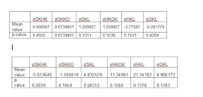
AES results Again

The AES results in the previous post were cut off, here they are again.

The top table is the AES for 1981-2002, the bottom table for 1989-2002.

Where my treatise is currently at

It has a been a while since I have posted. During that period I was working on my partial treatise draft, which I handed in on Friday and obtaining some preliminary results. In the partial treatise draft I had completed the introduction and motivation, literature review and methodology chapters. I had also presented some details on the data collection and some preliminary results. The first three chapters are no means complete and I will be refining them further along the weeks incorporating in the comments that I obtain from Dr.Poon.

Since the partial draft I have been further working on my results. The preliminary results which I have obtained so far are attached below. They include an estimation of the translog model for the 1981-2002 period and 1989-2002 period as well as the AES obtained for both periods.


Regression Results of Translog 1981-2002

Coefficients

Estimate

Std. Error

t value

Pr(>|t|)

βo

1.935069

4.095545

0.472482

0.637037

βSK

-3.59742

0.601137

-5.98435

8.40E-09

βHK

3.196295

0.540743

5.910936

1.24E-08

βOK

-3.08555

0.595171

-5.18431

4.79E-07

βL

4.412228

0.777771

5.672913

4.25E-08

βSKHK

-0.07981

0.056434

-1.41422

0.158668

βSKOK

0.29958

0.052916

5.661461

4.51E-08

βSKL

0.040585

0.030756

1.319565

0.18831

βKHOK

-0.25008

0.043943

-5.69116

3.87E-08

βHKL

-0.0316

0.026971

-1.17163

0.242572

βOKL

-0.36169

0.038045

-9.50682

2.96E-18

βSKSK

0.056274

0.028064

2.005184

0.046131

βHKHK

0.039415

0.030344

1.29895

0.195279

βOKOK

0.304332

0.038915

7.82046

1.97E-13

βLL

-0.00655

0.027073

-0.24209

0.808926

T1982

-0.07036

0.083668

-0.841

0.401232

T1983

-0.18504

0.088161

-2.09891

0.03693

T1984

-0.23224

0.094434

-2.45932

0.014667

T1985

-0.2968

0.101679

-2.91895

0.003866

T1986

-0.40875

0.108416

-3.7702

0.000208

T1987

-0.55139

0.11776

-4.68233

4.88E-06

T1988

-0.64727

0.124346

-5.20538

4.33E-07

T1989

-0.73405

0.127711

-5.74775

2.90E-08

T1990

-0.8428

0.132905

-6.3414

1.22E-09

T1991

-0.94061

0.136498

-6.89099

5.40E-11

T1992

-1.02249

0.139904

-7.30853

4.56E-12

T1993

-1.06997

0.142023

-7.53379

1.16E-12

T1994

-1.10585

0.143281

-7.71804

3.73E-13

T1995

-1.13752

0.143058

-7.95148

8.63E-14

T1996

-1.1319

0.143119

-7.90879

1.13E-13

T1997

-1.15017

0.143922

-7.99162

6.70E-14

T1998

-1.1646

0.146581

-7.94509

8.99E-14

T1999

-1.20425

0.150877

-7.98168

7.13E-14

T2000

-1.28412

0.158085

-8.12293

2.91E-14

T2001

-1.37719

0.162579

-8.47092

3.07E-15

T2002

-1.41934

0.167084

-8.49475

2.63E-15

Iservice

0.515471

0.038752

13.30167

3.11E-30


AES for 1981-2002

σSKHK

σSKKO

σSKL

σHKOK

σHKL

σOKL

Mean value

0.098557

0.6739457

1.209937

1.209937

-3.77287

-0.281779

p-value

0.4502

0.07933

0.3311

0.1038

0.1031

0.4289


Regression Results of Translog 1989-2002

Coefficients

Estimate

Std. Error

t value

Pr(>|t|)

βo

-2.76934

3.496849

-0.79195

0.429738

βSK

-4.91899

0.733963

-6.70197

4.73E-10

βHK

3.282922

0.436596

7.519358

6.17E-12

βOK

-3.70208

0.628954

-5.8861

2.82E-08

βL

6.466395

0.809478

7.988354

4.68E-13

βSKHK

0.254486

0.070287

3.620682

0.000411

βSKOK

0.317701

0.061771

5.143242

9.01E-07

βSKL

0.29704

0.043638

6.806945

2.74E-10

βKHOK

-0.22608

0.03697

-6.11539

9.20E-09

βHKL

-0.16539

0.029004

-5.7024

6.82E-08

βOKL

-0.37694

0.041219

-9.14489

6.61E-16

βSKSK

-0.21684

0.04987

-4.34821

2.64E-05

βHKHK

-0.05881

0.027685

-2.12441

0.035406

βOKOK

0.33207

0.042761

7.765808

1.60E-12

βLL

-0.13565

0.023766

-5.70765

6.65E-08

T1990

-0.13121

0.047436

-2.76602

0.006446

T1991

-0.24256

0.049593

-4.89092

2.74E-06

T1992

-0.32922

0.052037

-6.32657

3.21E-09

T1993

-0.36548

0.053528

-6.82791

2.46E-10

T1994

-0.38471

0.054356

-7.07753

6.62E-11

T1995

-0.39591

0.054812

-7.22317

3.05E-11

T1996

-0.37964

0.055736

-6.81141

2.68E-10

T1997

-0.37973

0.057315

-6.6253

7.03E-10

T1998

-0.36279

0.060596

-5.98709

1.73E-08

T1999

-0.39968

0.064078

-6.23743

5.02E-09

T2000

-0.46585

0.070161

-6.6397

6.53E-10

T2001

-0.57207

0.072914

-7.84578

1.03E-12

T2002

-0.61339

0.076199

-8.0499

3.33E-13

Iservice

0.508949

0.030608

16.62825

7.34E-35


AES for 1989-2002

σSKHK

σSKKO

σSKL

σHKOK

σHKL

σOKL

Mean value

-5.033649

-1.590819

4.832529

-11.34981

21.34182

4.966173

p-value

0.2039

0.1658

0.04353

0.1566

0.1376

0.1783


Two different time periods have been used since an accurate deflator for the data from 1981-1989 could not be obtained form the ABS. Since we had to estimate these numbers there is a strong possibility that we will introduce significant measurement error into the model. Since the data set being used in a panel data set i.e. a cross section of industries observed across time, the measurement error is attenuated in the model. Consequently our parameter estimates will be biased, inconsistent and inefficient and any inferences drawn about them will be invalid.

Dr.Poon has also asked me to estimate the translog model using random effects. The purpose of this is to check whether the fixed effect model we are currently using is a suitable choice via a statistical test called the Hausman test. However, this is not possible since we need to obtain the between estimator. The between estimator measures the variability between different industries. Since we are estimating 14 parameters but only have 12 industries we cannot obtain the between estimator. I have emailed Dr.Poon about this and am awaiting his reply as to how he would like me to proceed regarding this.


Dr.Poon has also asked me if could try and estimate another model called the Constant Elasticity of Substitution (CES) model using the Eview software package. The results of this model will then be compared to the translog model. I have tried to estimate this model but once again come across problems. The error that was being generated was that a near singular matrix was formed. This means that there is collinearity present and that there the regressors are dependent. I suspect that this is due to the high correlation between the Hardware Capital and Software Capital in excess of 85%. I have emailed Dr.Poon about this and am awaiting his reply.


I am also researching testing for aggregation error. My treatise is not just focused on testing the complementarity between Software Capital and other production inputs but also testing whether Software Capital and Hardware Capital can be aggregated into a single IT measure. The argument is that if these two production inputs are not perfect substitutes they cannot be aggregated into one measure since we will be omitting the complementarity that they add to business value. Dr.Poon has provided me with the following readings to review:

  • Aizcorbe, A. (1990) Journal of Business & Economic Statistics, 8, 373-383.
  • McGukin, R. H. and Stiroh, K. J. (2002) Economic Enquiry, 40, 42-59.
This week I am also working on a Presentation that Dr.Poon has asked each of his students to provide a presentation of their treatise progress so far. In my next post I will be providing details to the response of the problems I have encountered and hope to present some preliminary results of the tests for aggregation error.